![]() Home page
Home page
 Contact me! (diaz_sebastien@gmx.fr)
The subject of our training course having somewhat changed, we will not treat in an exclusive way the calibration of a thermometer with low temperature but of the construction of an automatic magnetic measurement setup [12T,2-300°K]. Indeed, our subject training course in the High Magnetic fields Laboratory (LCMI) was to set up a system of magnetization measurement on a superconductive coil which can generate a field of 12 Tesla. We will treat here various systems which we used. We will tell in a simplified way how you can measure a relatively weak magnetization compared to the field applied to the sample. Then we will explain how we proceeded to calibrate a resistive thermometer of semiconductor type, measuring temperatures between 1°K and 300°K. We will present the cryostat in which is located the measurement setup and the various thermal insulations which protect it from a reheating by the external medium. Finally the assembly will be described and we will give the result of a measurement of magnetization obtained on piece of Nickel (calibration).
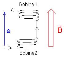
The principle of this measurement of magnetization consists in measuring the induced fem for the flux variation created by the displacement of materials magnetized through a closed loop.
Indeed, according to
the Faraday's law, the fem induced in a closed loop and "
motionless " is such as![]() With
f the flux of
With
f the flux of
![]() through this circuit, i.e.
through this circuit, i.e.
![]()
In the case of our
experiment we have
![]() parallel with the normal of surface and
parallel with the normal of surface and
![]() with
with
![]() field created by the superconductive coil and
field created by the superconductive coil and
![]() the
magnetization induced on the sample by this external magnetic field..
Therefore we have
the
magnetization induced on the sample by this external magnetic field..
Therefore we have
![]()
In order to
eliminate heterogeneity from the field
![]() ,two
compensated coils i.e. rises in reverse are used so that any
variation of induction results in a null flux variation.
,two
compensated coils i.e. rises in reverse are used so that any
variation of induction results in a null flux variation.
Therefore, if f
1 is the flux
of![]() through the two coils when the sample is located in the coil number
1, we have:
through the two coils when the sample is located in the coil number
1, we have:
f1=(m0 *(H+M)-m0 *H)*S
The same if f
2 is the flux of
![]() ,
when the sample is located on the second coil, we have :
,
when the sample is located on the second coil, we have :
f2=(m0 * (H+M)-m0 *H)*S
Therefore the induced fem during displacement is:
![]() with n=the number of whorls
with n=the number of whorls
This implies that by integrating the signal detected et the boundaries of the two coils, we obtain a size proportionnal to magnetization M.
Only, the signal that we measure is really very weak, this is why we do not use two coils in oppositions but four coils connected in opposition two by two. Thus, the component of the signal coming from the presence of a constant field is withdrawn better than with a system of two coils. A compromise thus has was made between the amplitude of the measured signal and the fact of not measured the continuous-current field H.
We present the signal we have obtained with our system of measurement:
The proportionality factor is given starting from an extraction of sampling, where we know magnetization M at saturation of the Nickel sample: M=m adze / M ol * 0.606*5585.
Where 0.606 m B is the saturation magnetization of Nickel and the 5585 convertion rates of the magnetons of bhor with emu.
But we will describe a little more the calibration of our measures to the part V of this report.
![]() Return to the contents
Return to the contents
Magnetization measured previously is connected to the temperature to which is subjected the sample. Among the most known samples, we knows that the variation of magnetization is a function of the temperature with constant external field. Here some curves presenting the behavior of susceptibility in four significant cases of magnetic nature:
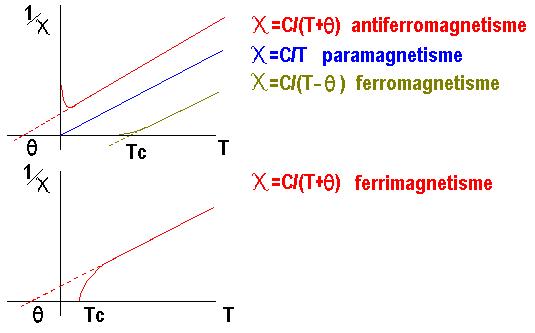
It is thus capital to have with precision the value of the temperature to which is the sample during measurement. For that, we will use a thermometer says secondary which will not give us access directly to the absolute temperatures because we does not measure thermodynamic properties. The thermometers most frequently used a reresistive or capacitive.
Among the resistive ones, onewe distinguish two main categories:
on the one hand the metal resistive thermometers whose conductivity answers the law of Drude :
s=Ne²t/m*
With: - m': effective mass
- n : number of electrons per unit of volume
- E : elementary charge
- T : time between two elastic collisions, this value is directly connected to the thermal agitation of the atoms thus at the temperature.
A resistance Rhodium-iron placed on the bottom of the tank enables us to know the temperature of the cryostat during cooling what provides us significant information. At the time of first cooling with nitrogen, the appearance of nitrogen liquid with atmospheric pressure causes a stage of temperature to 77°K we will note it thanks to a measurement of constant resistance to 6.753 W . Of the same, during cooling to helium, we will observe the stage of temperature to 4.2°K by a measurement of constant resistance to 1,89 W .
in addition, there are resistive thermometers semiconductor.
Here electric conduction will be a function of the aptitude of the electrons for being able to cross the energy band of gap separating the valence band from the tape of conduction; aptitude determined by the thermal energy of the system. It is the variation of the number of electrons in this tape of conduction, with the temperature which is at the origin of the variation of resistivity. Contrary to the metal resistive thermometers, where the resistivity increases when the temperature increases, the resistivity of the semiconductor type thermometer increases when the temperature decreases because the number of electrons able to cross this energy barrier is determined by the statistics of the Maxwell-Boltzmann.
In order to know the temperature of our sample, we placed a resistance CERNOX (standard semiconductor) in the cane sample (see diagram of the cryostat part three) which we calibrated before.
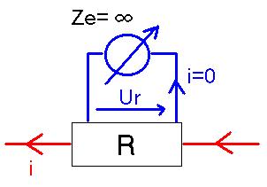
To calibrate a resistance, it is significant that we can have access to a precise and reliable measurement in spite of the constraints which utilizes such an experimentation. The first difficulty results in the distance obligatorily separating resistance from the measuring apparatus. The resistance of being useful wire to connect these two elements should not thus be measured with resistance(as we would have classically done with a measurement of the type two wire). To avoid that, we carry out a measurement of 4 wires resistivity. Two wire are used to make pass through a resistor a constant intensity than the two others wire are used to measure the tension of the resistor. From now on the majority of measurement setup present a direct reading of the resistance by the method of four wire.
An another constraint comes from the difficulty brought by cryogenics. So that the calibration of our resistance is valid, it is necessary to traverse the range of temperature going of 4°K to 300°K.
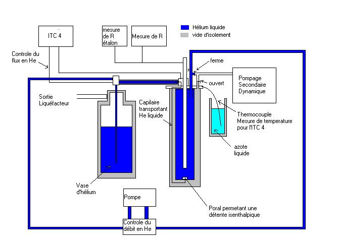
Diagram of the calibration setup
We will not explain the difficulties here that represent the use of helium liquid and the precautions that imposes. These various points will be detailed thereafter.
We will notice simply that the helium vaporized in the cryostat is aspired by the pump in order to facilitate the transfer of liquid helium by a slight depression in the cane of transfer. Then we reinjects it in the mud for a return towards the liquefier.
During handling, it does not remain any more that has to stabilize the temperature by regulating the PID (Proportional,Intégral, Dérivé) from the ITC4, and to measure the values of our resistance which we compare with the values of another cernox « préétalonné » in factory, that we placed near our resistance.
Thereafter, a polynomial regression on the curve of the reference resistor according to our resistor then on the temperature curve according to the reference resistor enables us to obtain an arithmetic relation connecting the temperature to measured resistance. So that the software of polynomial regression MicrocalOrigin5 can provide a result usable thereafter, we have to carry out a judicious cutting of our curves in several parts. These parts overlap at the ends so that the curve T=f(R), or rather T=g(ln(R)) in our case,varies continuously. The calibration curves which we have just mentioned are provided in appendix of this report/ratio.
Lastly, to facilitate the reading of the temperature, a Labview program was worked out to carry out conversion after reading of resistance by cable GPIB.
![]() Return to the contents
Return to the contents
The cryostat is composed of several parts of outside towards the interior we finds:
A secondary vacuum of insulation in order to avoid any heat exchange with outside and thus allowing to go down at temperatures which allow the appearance of liquid helium. Moreover, screens are placed so that the background radiation does not heat the interior of our tank.
A tank that one filled of liquid Helium is used for thermaliser with 4,2°K the reel creating the field. Such a temperature is necessary so that the coil is in its superconductive state. The user will be able to run a current going up to 88 Ampères to generate the field of 12 Tesla. If the coil is not sufficiently cold at the time of the rise in field, it is possible that this one forwards and has a resistance not negligible. This commonly named transition " quench", would cause total and fast evaporation of liquid helium. This phenomenon being brutal, we could note that it destroyed our system of measurement and that it could have deteriorated the superconductive coil.
A second vacuum of insulation separating the tank from the insert.
Another liquid helium tank, which we call the insert and which we use like cold source. While pumping on the helium output,we can reach temperatures lower than the Kelvin degree.
Always of outside towards the interior, we find initially the cane which carries the two coils of detection which soak in the liquid helium of the insert; what decreases the resistivity of copper, making the signal detected much less disturbed.
Then,we find the cane supporting the device of heating,composed of a wire of manganin of a total resistance of 124 W. Obviously, between the cane of " heating " and the cane of detection,we have a vacuum of 10 -5 mmHg for avoiding heating the liquid helium of the insert. However, so that the sample can be has a temperature bordering the degree Kelvin a metal ring cylindrical is inserted between these two canes, which allows a thermal conduction between the sample and the insert.
Lastly, we find the cane carries sample where is the thermometer which is resistance that one calibrated previously.
To be able to fill the liquid helium cryostat, without using much helium, it is initially necessary to make cold the 2 tanks with nitrogen liquid in order to lower the temperature of the cryostat to 77 °K.
After having waited until all the interior of the cryostat was thermalised at this temperature, we drive out nitrogen liquid by sending air under pressure in the tanks. Once that all, the liquid nitrogen evaporated, we pump the gas which it remains inside the tanks in order to avoid that it does not freeze during the liquid transfer of helium. This could stop the outputs;that which would create over pressures.
Once that the vacuum is made, we make re-enter of gas helium then we traps gently.
Like the helium transfert is done by the bottom of the cryostat, from the cold helium vapor initially will cool the coil and the tank. Thereafter signs, like the reheating of the discharge pipes of helium, i.e. the evaporation of condensation, show us that the first helium drop has just appeared at the bottom of our cryostat.Moreover resistor Rhodium iron to the bottom of the cryostat always brings to us the significant indications during the filling. The tank is thus brought up to a temperature of 4,2°K, which is the temperature of liquid helium.
Thereafter to use a magnetic field of 12 Tesla we must take some precautions concerning the security of the assembly and the users.
Indeed, the proximity of the field is prohibited to all people carrying a pacemaker. In the same way, the user will have to remove any object likely to answer the field because it would thus be likely to cross the part and to cause by the same occasion of the dégats. Finally any magnetic medium a such blue card will have to be put at the variation not to be demagnetize. We could note during measurement that a screen of cathode ray tube computer can undergo a modification of its display and that it is thus advised to use a liquid crystal display.
![]() Return to the contents
Return to the contents
Limps of feeding will have to thus function as follows:
By the application of a signal TTL of 5 volts the engine must start to go down until the sensor of bottom commutates and goes from the logical position 1 to 0.
Then the engine will not have to go up as long as signal TTL will not have to taled zero.
Finally the engine will have to stop when the sensor top commutates and goes from the logical position 1 to 0.
Logical drawing :
The engine is supplied by a source of tension of 24 V between 4 transistors of power controlled by a logical circuit; what enables us to reduce to mount or the engine without changing the polarity of the feeding.
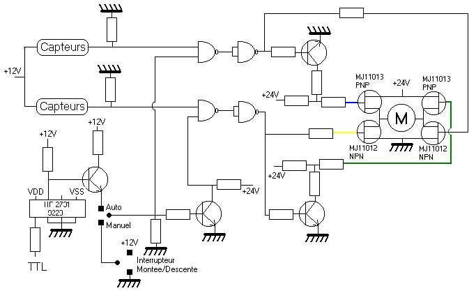
diagram of the logical circuit which feeds it limps
We thank Mr. Plante who helped us to regulate the problem of compatibility between the two types of sensors and which corrected some of our errors.
![]() Return to the contents
Return to the contents
Now that the various parts necessary to our assembly were worked out, it is necessary for us to join together them in order to begin our measurements.
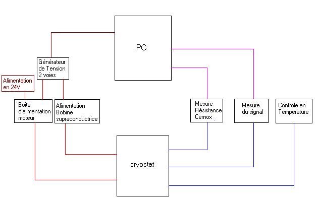
diagram presenting the various ones connected connecting the apparatuses between them
The various cables GPIB which we can notice will connect the various measuring apparatus to the computer in order to be able to take a measurement simply. Thanks to programming in the Labview language, it will be possible to the user to control all the apparatuses since a computer.
Indeed, the programming is relatively simple thanks to thepresentation of the various functions, loops, tools... in the shape of icons or drawings. These icons are then connected by wire which determine the way in which will be carried out the program.
Thus, a program entitled initialisation.vi will communicate with the various measuring apparatus and will order to them to ber egulated on the desired gauge of measurement. The superconductive coil not being able to support a variation in too fast intensity, the control program of field named field command.vi has three fonctions.It determines the intensity has to provide to the coil to reach the wished field, measurement the intensity which crosses already the coil, then varies in the direction wished without exceeding the speed of maximum variation of 3 Tesla per minute. This program is that which we present in appendix as a sample program that we have to carry out under Labview.
Finally the last sample program that we will see will be that which measures magnetization according to the value in field. The user will determine the various stages in field which it wishes to make, then the number of extractions of the sample by stage. Once the few adjustments finished, the program controls the intensity sent through the coil, then place in a table the values of the temperature of the sample, the value of the field, and the magnetization which presents the sample during the extraction. An average by stage is automatically calculated and recorded in a second file. Moreover this program makes it possible to visualize the shape of the signal (graph in part I), the user can thus control if the measurement which it has just taken is valid, too disturbed,or still not centered compared to the detection coils.
As explained previously, the signal was integrated and we added integration on the descent to integration on the rise. Only the value of integration thus obtained is not yet great interest since the unit is purely whimsical. We must thus calibrate our detection coils. For that, we will use a Nickel sample whose purity is 99.999% and of which the thickness is weakest possible in order to be small in front of our measuring apparatus. The calibration is done starting from Nickel because this metal has as characteristic to have a ferromagnetic behavior which is saturated with relatively weak field, typically near the Tesla.
We present the curve to you representing themagnetization of a piece of Nickel cylindrical height 1.88mm and ofmass 1.0922g obtained to the LCMI on the assembly describes in this report:
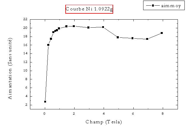
It will be noticed that magnetization according to the field with saturation is not exactly a horizontal curve. Since the electrons present a spin equal to ½, one can expect an increase in magnetization by alignment with the field and this, even after saturation. On the curve which one can observe we notices that it is not a question here of an increase but of a reduction. We can propose two reasons with this phenomenon:
a magnetic spectrum of moment opposed to the sample appears in the matter supraconducting and decreases measured magnetization.
a noise which increases with the field and which we chose to not consider, the number of point of measurement which we just decreases with the increase in the field.
By a prolongation of the right-hand side towards the null field, we can deduce magnetization from saturation of Nickel without the increase in the electrons of conduction with the field not intervening. This magnetization will be compared with that which we can calculate in a theoretical way thanks to knowledge of the mass of the sample, its molar mass and its magnetization of saturation per mole. For Nickel, the saturation magnetization is 0.606 m B per mole and the molar mass is of 58.71g/mole. By a simple calculation one finds a value theoretical of the magnetization of 11.2736*10 -3 m B is 62.963 moved.
![]() Return to the contents
Return to the contents
Although we did not work with the same orders of magnitude in field and temperature, the work practise « Newton » brought most of knowledge necessary to us, to the comprehension and the assembly.
During this training period,we have learned to use numerus technic as secondary pumping by an oil diffusion pump, or various aspects of cryogenics and handling of liquid helium. Finally this training course will have enabled us to attend and take part a measurement of magnetization with a field external of 26 Tesla.
We thank the High Magnetic Field Laboratory, and more particularly Professor Chouteau and his team for their greeting, to have allowed us to make this training course and to have helped us in the assembly of this measuring apparatus
![]() Return to the contents
Return to the contents
![]() Return to the Home Page
Contact me! (diaz_sebastien@gmx.fr)
Return to the Home Page
Contact me! (diaz_sebastien@gmx.fr)
Last modification :